Introduction to Programming for Public Policy (30550)
Weather and Crime
The Question
This project is an exploration of the interaction of weather and crime in Chicago. It is initially motivated by the strong seasonal variation observed the crime rate for Chicago. By presenting stable crime rates for cities without cold winters, I suggest that temperature – rather than daylight or summer schedules – is the relevant pathway for this seasonal effect. In the context of a regression for Chicago crime, the coefficients on temperature and precipitation are large and significant. I thus reproduce earlier results in this realm. After removing the secular trends over time, temperature is responsible for around 60% of the residual variation in the rates of battery, theft, and assault.
Towards the end of the investigation, I analyze the outliers in the distribution and suggest various alternative specifications. I evaluate which types of crime are most related to temperature.
Past Work
Past work has validated the intuitive premise that crime rises with temperature. Recent studies by Ranson, and Gamble and Hess in the context of climate change have found strong positive correlation of temperature with crime. Both find that the slope falls with increasing temperature. However, these and earlier work by Field (1992) were at the monthly level. This project benefits from more-precise data and probes daily variation in temperature and precipitation. Field’s work at the monthly level for England and Wales failed to identify a significant effect of rainfall, whereas the daily analysis presented here finds a stark effect.
Data
Check-out scripts for the data in this analysis can be found in my data repository.
City Crime Data
I have downloaded data from 10 major US cities with public crime data portals that report crimes with a time and location. While I focus the analysis on Chicago, I do use data from Dallas, San Francisco, Phoenix, and Philadelphia to separate out seasonal variations from temperature variation. The datasets used are:
- Chicago
- San Francisco
- Dallas
- Phoenix
- Philadelphia
- Los Angeles
- Portland
- New York City
- Boston 2012-2015 and 2015-present
- Denver
A check-out script for all of these data is found here:
The reporting periods vary widely between cities. Records in Chicago and San Francisco go back to 2001 and 2003; while those for Dallas and Phoenix start in just 2014 and 2015. The definition of crimes also varies. For example Chicago and Philadelphia report crimes, New York reports seven major felonies, Phoenix reports nine major felonies, and San Francisco and Dallas include non-criminal responses. I remove non-criminal offenses in the analysis.
I could also have used the FBI’s Uniform Crime Reports, but these are aggregated to the monthly level.
Weather Underground API
The Weather Underground API provides an outstanding interface for retrieving historical weather data:
- https://www.wunderground.com/weather/api/
The service provides hourly weather data for major US airports at the hourly level, dating further back than any of the crime datasets. A free account provides 500 calls per day and 10 calls per minute. Each call returns one day worth of day, usually with 24 hourly observations. A script is provided that downloads one airport and year (365 calls, every 7 seconds), and which can be run daily:
This script retains the complete json response for each call,
and also extracts a daily csv “reduction,”
that includes only the observation times, temperatures, and precipitation.
It is then trivial to cat together a complete record for a city.
I have downloaded complete records for Chicago and Phoenix.
Investigation
All analysis code for this project is included in a single jupyter notebook:
The bulk of the analysis is performed in python, pandas and statsmodels, but I do use command line tools to reduce the data volume. These calls are also contained within the notebook.
Comparison of Cities
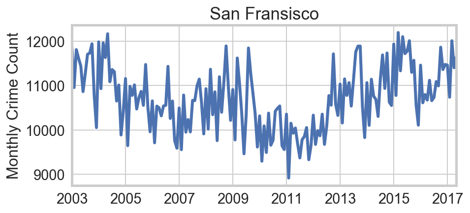
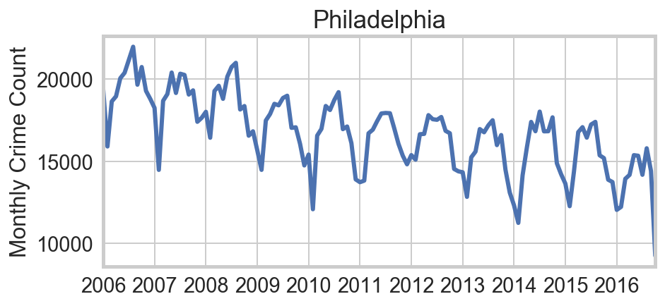
The observation that motivates this analysis is the strong seasonal variation in Chicago crime rates, which correlates in an obvious way with temperature:
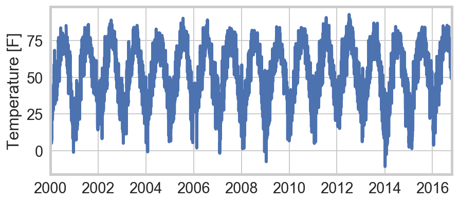
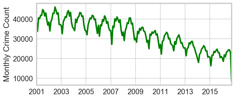
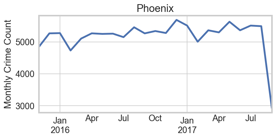
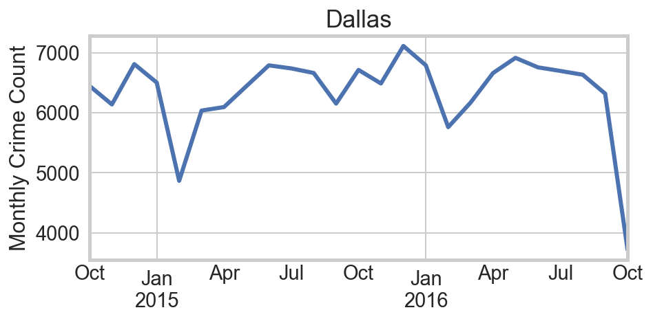
The first question is whether temperature is truly the “culprit,” or if instead the variation is simply seasonal. Are we simply seeing more kids off from school? Or more houses unattended while families take vacations? Or longer evening hours? Winters in San Francisco, Phoenix, and Dallas are far less severe than Chicago, and they exhibit no notable annual cycles in crime rates. By contrast other northern cities like Philadelphia do. This provides strong circumstantial evidence that temperature is the relevant factor.
Regression Analysis
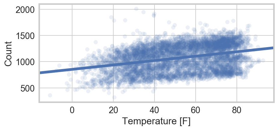
The initial regression to report is simply daily crime rates on average (daily) temperature in Chicago. The regression displays a very clear trend but enormous, non-normal residuals.
The obviously missing factor is the secular reductions in crime since reporting began. To address this, yearly fixed effects and a linear time trend are almost equally effective. I choose the non-parametric approach (fixed-effects).
The Baseline Model
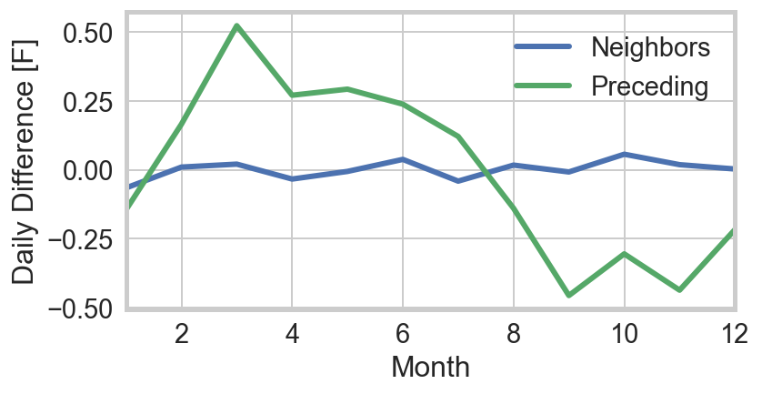
In addition to the secular trend, we have seen before that crime rates exhibit strong weekly cyclicity. I therefore include both yearly and day-of-week fixed effects. I also include a dummy for precipitation. The main item of interest is the coefficient on the temperature. Because I am curious as to the effect of hot relative days, I also include the difference in the daily average with the average of the days before and after. I use the average of both neighboring days instead of simply the preceding day, to ensure that the variable is distributed around zero. Looking simply at the difference with respect to the preceding day shows seasonal fluctuations as on average it gets warmer in the spring and cooler in the fall.
All in all, with year y, day of week w, temperature T, and “daily difference” as DD, the the model is:
Crime ~ αyw + βTT + βDDDD
The results are as follows:
| Dep. Variable: | NC | R-squared: | 0.888 |
|---|---|---|---|
| Model: | OLS | Adj. R-squared: | 0.887 |
| Method: | Least Squares | F-statistic: | 1884. |
| Date: | Sat, 30 Sep 2017 | Prob (F-statistic): | 0.00 |
| Time: | 22:14:03 | Log-Likelihood: | -33576. |
| No. Observations: | 5750 | AIC: | 6.720e+04 |
| Df Residuals: | 5725 | BIC: | 6.737e+04 |
| Df Model: | 24 | ||
| Covariance Type: | nonrobust |
| coef | std err | t | P>|t| | [0.025 | 0.975] | |
|---|---|---|---|---|---|---|
| Intercept | 1081.4429 | 6.049 | 178.778 | 0.000 | 1069.584 | 1093.301 |
| C(Yint)[T.2002] | 4.1555 | 6.199 | 0.670 | 0.503 | -7.997 | 16.308 |
| C(Yint)[T.2003] | -14.6876 | 6.200 | -2.369 | 0.018 | -26.841 | -2.534 |
| C(Yint)[T.2004] | -40.2627 | 6.194 | -6.500 | 0.000 | -52.405 | -28.120 |
| C(Yint)[T.2005] | -86.5471 | 6.198 | -13.964 | 0.000 | -98.697 | -74.397 |
| C(Yint)[T.2006] | -103.9345 | 6.197 | -16.772 | 0.000 | -116.083 | -91.786 |
| C(Yint)[T.2007] | -129.3048 | 6.197 | -20.864 | 0.000 | -141.454 | -117.155 |
| C(Yint)[T.2008] | -148.2334 | 6.197 | -23.920 | 0.000 | -160.382 | -136.085 |
| C(Yint)[T.2009] | -238.5630 | 6.203 | -38.458 | 0.000 | -250.724 | -226.402 |
| C(Yint)[T.2010] | -313.0629 | 6.197 | -50.516 | 0.000 | -325.212 | -300.914 |
| C(Yint)[T.2011] | -360.6227 | 6.198 | -58.179 | 0.000 | -372.774 | -348.471 |
| C(Yint)[T.2012] | -425.2000 | 6.195 | -68.640 | 0.000 | -437.344 | -413.056 |
| C(Yint)[T.2013] | -477.9702 | 6.200 | -77.098 | 0.000 | -490.124 | -465.817 |
| C(Yint)[T.2014] | -561.6879 | 6.202 | -90.571 | 0.000 | -573.845 | -549.530 |
| C(Yint)[T.2015] | -608.9072 | 6.197 | -98.254 | 0.000 | -621.056 | -596.758 |
| C(Yint)[T.2016] | -621.5207 | 6.657 | -93.357 | 0.000 | -634.572 | -608.469 |
| C(DoW)[T.1] | 19.9642 | 4.110 | 4.857 | 0.000 | 11.906 | 28.022 |
| C(DoW)[T.2] | 28.6811 | 4.110 | 6.979 | 0.000 | 20.624 | 36.738 |
| C(DoW)[T.3] | 19.0278 | 4.111 | 4.628 | 0.000 | 10.968 | 27.088 |
| C(DoW)[T.4] | 78.4653 | 4.114 | 19.075 | 0.000 | 70.401 | 86.529 |
| C(DoW)[T.5] | 17.6794 | 4.112 | 4.299 | 0.000 | 9.618 | 25.741 |
| C(DoW)[T.6] | -43.8975 | 4.112 | -10.676 | 0.000 | -51.958 | -35.837 |
| C(P)[T.True] | -29.8673 | 2.377 | -12.564 | 0.000 | -34.527 | -25.207 |
| T | 4.5349 | 0.058 | 78.593 | 0.000 | 4.422 | 4.648 |
| DD | -0.9165 | 0.251 | -3.656 | 0.000 | -1.408 | -0.425 |
The model has a high R² of 0.89.
- The yearly fixed effects show spectacular yearly reductions in crime, over the past fourteen years.
- The day-of-week fixed effects show crime peaking on Friday (4) and at its lowest on Sundays (6), as usual.
- Temperature is positively and extremely significantly associated on crime (t = 79).
- Precipitation is associated with a large and highly significant (t = 13) reduction in the daily crime rates.
- These estimates are so large that there is no doubt as to that weather is associated with rates, and little need for more-subtle tests. Nevertheless, alternative specifications can alter somewhat the values of of the coefficients.
- I would argue that these effects are plausibly causal, given the evidence from other cities.
- The coefficient on the “daily difference” is negative and moderately significant, but for alternative specifications can be consistent with 0.
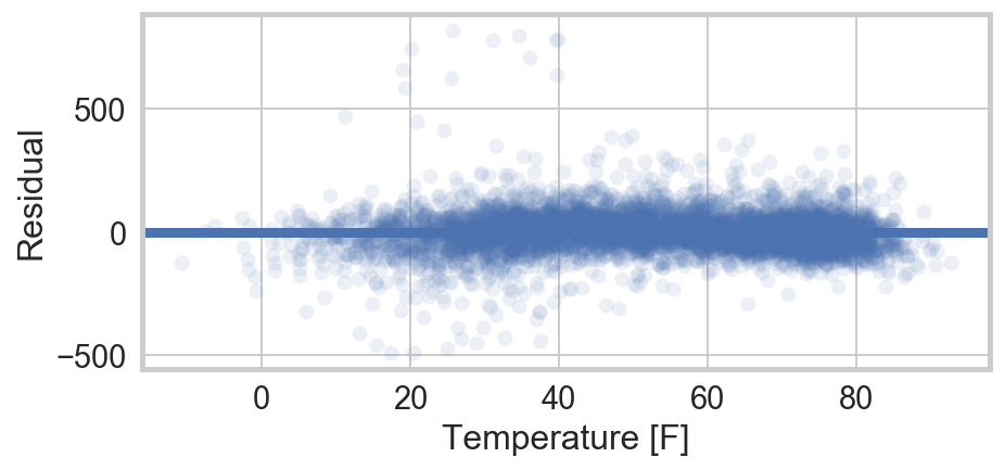
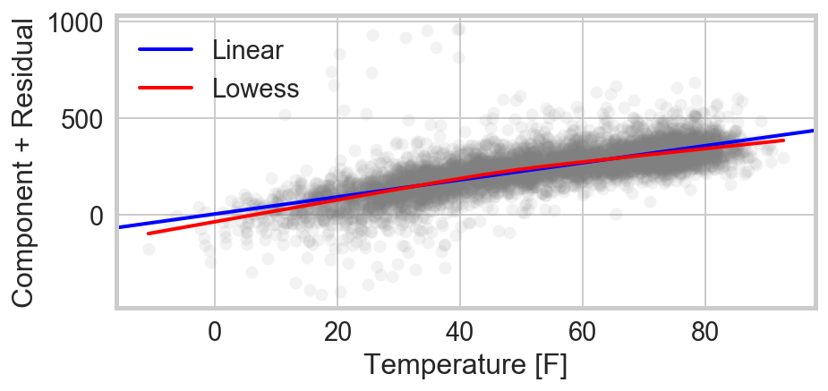
Observations on the Residuals
The residuals of the elaborated model are dramatically tighter than the original temperature v. crime fit. However, at low temperature they are non-normal and tend to be negative. Fitting a non-parametric, locally-weighted linear regresion to the component + residual data, the slope of the fit line indeed falls with temperature. This confirms the intuition that “at a certain point, even criminals start to melt.” This behavior has previously been observed, in the work noted above.
Also notable in the residuals is the presence of a dozen or so outliers, with crime levels far from the trend and outside the distribution. We now turn to those days with more than 400 more crimes than nominally predicted.
Outliers Identified: New Year’s Day.
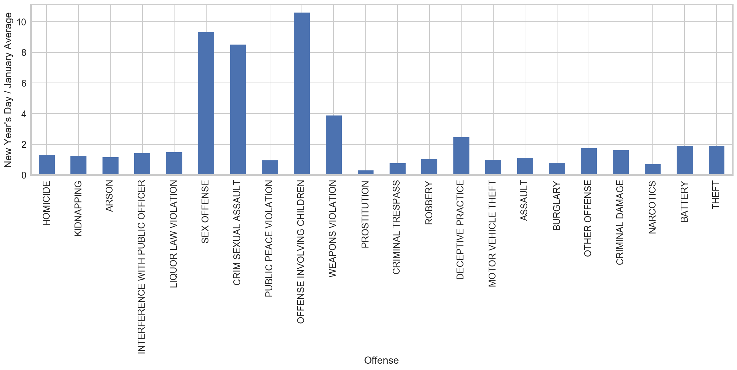
It turns out that every single one of these days is a New Year’s Day (2002-2015). One might naturally worry about a data reporting issue: some crimes that did not have a definite time, could simply be set to January 1. This does not appear to be the case. Although there is a spate of crimes at midnight, this appears to correspond to reporting at the end of the shift – not to a technical problem. Comparing the crime rate on New Year’s to the rest of the month, we see a fairly uniform rise in the rate across types. In particular, the normal “heavy hitters” of theft and battery have high ratios with respect to the normal expectations for January and make up for the bulk of the increase. The additional crime is not concentrated in, for instance, financial crimes, that might have different reporting procedures.
| Offense | January | NYD | ratio | |
|---|---|---|---|---|
| 0 | THEFT | 99632 | 6107 | 1.900163 |
| 1 | BATTERY | 82358 | 5034 | 1.894825 |
| 2 | NARCOTICS | 60640 | 1398 | 0.714677 |
| 3 | CRIMINAL DAMAGE | 51790 | 2677 | 1.602375 |
| 4 | OTHER OFFENSE | 34592 | 1953 | 1.750202 |
| 5 | BURGLARY | 28125 | 718 | 0.791396 |
| 6 | ASSAULT | 26698 | 957 | 1.111207 |
| 7 | MOTOR VEHICLE THEFT | 25005 | 803 | 0.995521 |
| 8 | DECEPTIVE PRACTICE | 19260 | 1527 | 2.457788 |
| 9 | ROBBERY | 18942 | 636 | 1.040862 |
Nevertheless, there are a few notable exceptions: crime types with increases far above the global increase of ~80%. Namely, there are overwhelming spikes in sexual crimes and crimes involving children.
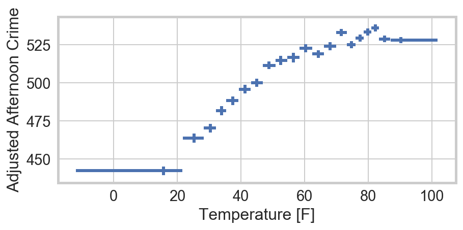
A Non-Linear Model
Next, we turn to a non-linear model for crime, as suggested by the non-normal residuals. Since I am particularly interested in identifying the turn-over where it might get “too hot for crime,” I focus here on crime in the afternoon (from noon to 6pm), when it might really get “too hot.” I allow for a linear coefficient for the year. We can see the effect we are trying to fit either by plotting a profile plot of the temperature after subtracting off the trend in the year, or by plotting the component plus residuals of a Count ~ Year + Time model. In both cases, there is an apparent change in the slope at around 50° F.
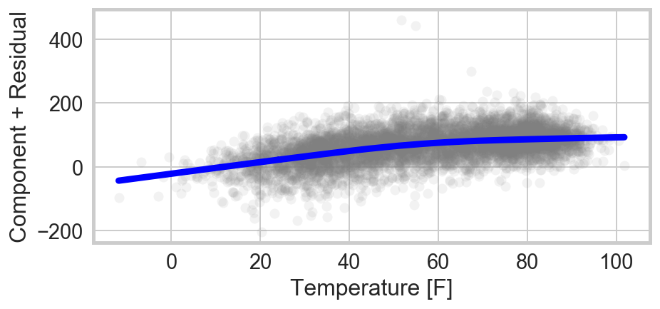
Since statsmodels isn’t built for this type of fit, I have used lmfit
to fit a piecewise function with

The model indeed fits a drop in the slope at 51.7±1.6° F, from 2.0±0.1 to 0.6±0.1 crimes per degree fahrenheit.
Alternative specifications for this behavior, for example as a quadratic, did not reliably converge.
Note that as specified, this model still fits a single absolute reduction in crime across years,
rather than a percentage fluctuation.
The latter specification would potentially be more appropriate, but is not natural with statsmodels.
The Most-Susceptible Types of Crime
Finally, it is natural to ask if there are specific type of crimes that are more-susceptible to the temperature than others. For this, I calculate the partial regressions on the residuals of the crime ~ year fit, for the 20 most common types of crime. I tabulate the ten crime types (of the 20 common types) with the highest partial correlations after removing the secular, yearly trend. For each of battery, assault, and theft, the correlations is around 60%.
| Offense | R | p | |
|---|---|---|---|
| 0 | BATTERY | 0.604118 | 0.0 |
| 1 | ASSAULT | 0.587209 | 0.0 |
| 2 | THEFT | 0.522527 | 0.0 |
| 3 | CRIMINAL DAMAGE | 0.506202 | 0.0 |
| 4 | GAMBLING | 0.416715 | 0.0 |
| 5 | ROBBERY | 0.355936 | 0.0 |
| 6 | BURGLARY | 0.312967 | 0.0 |
| 7 | PUBLIC PEACE VIOLATION | 0.267490 | 0.0 |
| 8 | WEAPONS VIOLATION | 0.256215 | 0.0 |
| 9 | MOTOR VEHICLE THEFT | 0.174238 | 0.0 |
Conclusions
This study reproduces past results that find increases in crime rates with temperature. By using crime and weather data aggregated at daily frequency, we also find tha precipitation puts a strong brake on crime. The crimes most susceptible to this temperature effect are battery, assault, theft and criminal damage. After accounting for the secular trends in crime rates, temperature is responsible for more than half of the remaining variation in the daily rates of these crime types, in Chicago.
We have explored alternative specifications, and confirmed that there is indeed a “ceiling” on this effect: higher temperatures correlate with higher crime, but the effect is smaller for days that are already very hot.